Table 2 presents the baseline characteristics of the discovery and validation cohorts used in the training, validation, and test datasets. The total number of data points is 953, divided into 571 for the training data, 191 for the validation data, and 191 for the test data. The dataset includes a variety of vehicle attributes, which are essential for the prediction of fuel efficiency. The “Vehicle type” attribute is divided into “car” and “van” categories. For the training data, 556 vehicles are classified as cars (97.4%), and 14 vehicles as vans (2.6%). In the validation and test datasets, the proportions remain similar, with 183 cars (95.8%) and 7 vans (3.7%) in the validation data, and 183 cars (95.8%) and 7 vans (3.7%) in the test data. The “Manufacturer/importer” attribute includes several brands. For the training data, 198 vehicles are from Kia (34.7%), 345 from Hyundai (60.4%), and a few from other manufacturers. In the validation data, 77 vehicles are from Kia (40.3%) and 109 from Hyundai (57.1%), while in the test data, 86 vehicles are from Kia (45.0%) and 108 from Hyundai (56.5%). The “Fuel type” attribute includes LPG, diesel, and gasoline. Most of the vehicles in all datasets use gasoline, with a few using LPG and diesel. The fuel type distribution is consistent across the datasets, with a slight variation in the number of diesel vehicles. The “Transmission type” attribute includes automatic and manual transmissions. The majority of vehicles across all datasets are equipped with automatic transmissions, with automatic types 4, 5, 6, and 8 being the most common, while a smaller proportion of vehicles have manual transmissions. The “Grade” variable is used to categorize vehicles based on their overall performance and fuel efficiency. The “light type” and “normal type” grades are the most common, with other grades showing fewer vehicles. Additionally, vehicle attributes such as engine displacement, combined CO2 emissions, tire inch size, and rolling resistance coefficient (RRC) were recorded for each vehicle. These variables are crucial as they directly impact fuel efficiency predictions. For example, the combined CO2 emissions for the training data are 161.5 g/km (28.5 standard deviation), which provides insight into the average environmental impact of the vehicles in the dataset. Finally, the “Combined fuel efficiency” variable, which measures the vehicle’s fuel efficiency in terms of the fuel consumption rate, is also included in the dataset. The average combined fuel efficiency for the training data is 12.00 (2.00), and the values for the validation and test datasets are similar, with slight variations in the standard deviations.

Analysis of correlation between two variables using CCA. (a) combined mode_CO2 and combined fuel efficiency analysis, (b) grade and combined fuel efficiency analysis, (c) transmission type and combined fuel efficiency analysis, and (d) vehicle type and combined fuel efficiency analysis.
Table 3 and Fig. 3 together illustrate the correlation analysis between combined fuel efficiency and various predictor variables, using Pearson, Spearman, Kendall correlation coefficients, and Canonical Correlation Analysis (CCA). Both analyses reveal that “combined mode CO2” and “grade” have consistently strong correlations with combined fuel efficiency across all coefficients (e.g., r = 0.88 and r = 0.89 in CCA, respectively, both with p = 0.000). This high degree of correlation suggests that these variables are critical in predicting fuel efficiency, as they have a substantial impact on outcomes. However, their strong correlation also raises concerns about potential multicollinearity, which could affect model stability if not carefully managed. In contrast, variables such as “transmission type” and “vehicle type” show weaker correlations with fuel efficiency, with r-values of 0.19 and 0.09, respectively, indicating that these factors may have limited predictive value and a smaller impact on fuel efficiency variation. The results of this combined analysis guide the selection of features in our predictive model: highly correlated variables like “combined mode CO2” and “grade” are prioritized for their predictive power, while lower-priority variables with weaker correlations can be deprioritized or excluded, thereby reducing model complexity and addressing multicollinearity risks.
We conducted a comparative study on the fuel efficiency of vehicles from Hyundai and Kia using statistical tests as summarized in Table 4. The t-test revealed a significant p-value of 0.00000605, indicating a substantial difference in the average fuel efficiency between the two manufacturers. This result suggests that consumers who prioritize fuel economy might find Hyundai vehicles to be a more advantageous choice compared to Kia, highlighting the importance of fuel efficiency as a key decision factor when selecting a vehicle. On the other hand, the Chi-squared test yielded a p-value of 0.572, indicating no significant difference in the distribution of vehicle types between Hyundai and Kia. This finding implies that both manufacturers have a similar range of vehicle types, such as SUVs and sedans, suggesting comparable competitiveness. Therefore, consumers searching for specific vehicle types may find suitable options available from both manufacturers, which could influence their purchasing decisions and marketing strategies. These insights provide valuable information for understanding consumer behavior and the competitive landscape between manufacturers. Automakers can leverage this data to enhance vehicle performance or refine their marketing messages, thereby appealing more effectively to their target audience. Overall, this analysis serves as a foundation for future research on fuel efficiency and vehicle type preferences, contributing to more informed decision-making by consumers and manufacturers alike.
Tables 5 and 6 present the evaluation results of six machine learning regression models, including both tree-based models (Extra Trees Regressor26, Random Forest Regressor27, Gradient Boosting Regressor21, Hist Gradient Boosting Regressor28, and AdaBoost Regressor29) and a linear model (Linear Regression8).
Table 5 shows the performance when using the full set of features and the performance when two highly correlated features, ’class’ and ’multimodal CO2’, were removed from the set to address multicollinearity. This adjustment was intended to assess the robustness of each model in dealing with potential collinearity issues. The results indicate that Extra Trees Regressor26 and Random Forest Regressor27 consistently outperform other models in terms of MSE, RMSE, and MAE values, with \(R^2\) scores closest to 1, both in validation and test sets. These models consistently show high performance even when multicollinearity is reduced, showing that they can reliably handle complex interrelationships in the data. On the other hand, the linear model showed significantly lower performance and was not stable.
Additionally, the K-Fold cross-validation metrics in Table 6 reinforce the reliability of Extra Trees Regressor26 and Random Forest Regressor27, showing stable and high accuracy across multiple data folds. This consistency underscores the robustness of these models, making them preferable choices for fuel efficiency prediction in this dataset.
Table 7 presents a comparative analysis of the performance metrics of the Extra Trees Regressor26 and Random Forest Regressor27 for Hyundai and Kia vehicles. In the validation data analysis, the Extra Trees Regressor26 achieves a minimum MSE of 0.007 for Hyundai, indicating excellent predictive performance, with a high \(R^2\) value of 0.998. This suggests that the model effectively predicts fuel efficiency for Hyundai vehicles. In contrast, the Random Forest Regressor27 has slightly higher MSE values for both manufacturers, indicating lower accuracy. Examining the test data, the Extra Trees Regressor26 records an MSE of 0.011 for Hyundai and 0.218 for Kia. The Random Forest Regressor27 shows MSE values of 0.017 for Hyundai and 0.315 for Kia. The \(R^2\) values are 0.960 for Hyundai and 0.980 for Kia, emphasizing the models’ efficiency. This analysis reveals that the Extra Trees Regressor26 consistently outperforms the Random Forest Regressor27 for Hyundai vehicles, suggesting it better captures the feature interactions specific to this manufacturer. However, the higher prediction errors for Kia indicate potential areas for optimization in the predictive model or vehicle design.

Actual vs Predicted values for fuel efficiency prediction models. (a) Extra Trees Regressor26, (b) Random Forest Regressor27, (c) Gradient Boosting Regressor21, (d) Hist Gradient Boosting Regressor28, (e) AdaBoost Regressor29 and (f) Linear Regression8.

Residual plots for fuel efficiency prediction models. (a) Extra Trees26, (b) Random Forest27, (c) Gradient Boosting21, (d) Hist Gradient Boosting28, (e) AdaBoost29 and (f) Linear Regression8.
In addition to the performance metrics presented in Tables 5 and 6, Figs. 4 and 5 offer a comprehensive visual analysis of model performance by comparing the actual versus predicted values and examining the residual distributions for each machine learning model used for fuel efficiency prediction, using all available features.
Figure 4 illustrates the Actual vs Predicted values, which provide insight into each model’s accuracy in replicating real-world fuel efficiency data. In this figure, data points that closely align with the red diagonal line indicate high prediction accuracy. The Extra Trees Regressor26 and Random Forest Regressor27 models show data points tightly clustered along the diagonal line, suggesting their effectiveness in capturing complex patterns across the dataset. AdaBoost29, on the other hand, shows a wider spread, suggesting it may be less accurate due to its sensitivity to noisy data and potential issues with overfitting. Figure 5 shows the residual distributions for each model, which help in understanding the bias and variance in predictions. Ideally, residuals should be symmetrically distributed around zero with minimal variance, indicating unbiased and reliable predictions. Both Extra Trees Regressor26 and Random Forest Regressor27 have residuals that are tightly centered around zero, confirming their accuracy and low bias as seen in Fig. 4. The Hist Gradient Boosting28 and Gradient Boosting21 models also show centralized residuals, but with slightly wider distributions, indicating a modest increase in variance. AdaBoost29 and Linear Regression8 exhibit wider and more dispersed residuals, with Linear Regression8 showing more variability due to its simplicity in capturing complex relationships within the dataset. These visualizations reinforce that tree-based ensemble models, such as Extra Trees26 and Random Forest27, are particularly effective for this dataset when all features are included. The close alignment of predictions with actual values and minimal residuals highlights the ability of these models to handle complex relationships. This suggests that ensemble models are well-suited for capturing the nuances of fuel efficiency prediction without the need for feature reduction in this case.
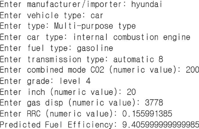
Example of fuel efficiency prediction system. (a) User input, (b) Fuel efficiency prediction value output.
The fuel efficiency prediction system was implemented based on the Extra Trees Regressor model26, which showed the highest performance. Figure 6 is an example of a fuel efficiency prediction system. As shown in Fig. 6a, by entering vehicle information such as manufacturer/importer, car type, fuel type, and transmission type, the fuel efficiency of the vehicle was predicted. In the example, the fuel efficiency was predicted to be 9.4.
Table 8 presents the results of the univariate analysis, showing the odds ratios and p-values for each variable related to vehicle fuel efficiency. The odds ratio quantifies the strength of the relationship between a given factor and fuel efficiency. Variables with a high odds ratio indicate a stronger impact on fuel efficiency, while those with a low odds ratio suggest less influence. For instance, fuel type has an odds ratio of 1.333, indicating a positive influence on fuel efficiency, where certain fuel types like diesel or LPG are associated with better fuel economy compared to gasoline. This underscores the relevance of considering fuel type when evaluating vehicle efficiency, as it significantly alters the model’s predictive accuracy. On the other hand, vehicle type has an odds ratio of 0.797, implying that specific vehicle types (such as vans) are less efficient than others, possibly due to factors like weight and design, which may increase fuel consumption. Transmission type also plays a significant role, with an odds ratio of 1.325, suggesting that automatic transmissions generally correlate with better fuel efficiency than manual ones. This relationship might be attributed to the optimization of fuel consumption in automatic transmission systems, which are designed to adjust shifting patterns for better fuel use. The significant effect of combined mode CO2 (with an odds ratio of 0.951) confirms that vehicles with lower emissions tend to have higher fuel efficiency. This result highlights the critical importance of reducing CO2 emissions to improve the overall fuel efficiency of vehicles and reduce their environmental impact. The p-values in Table 8 provide further confirmation of these findings, with fuel type, transmission type, combined mode CO2, and grade all showing highly significant relationships with fuel efficiency (p < 0.05). This statistical significance implies that these variables must be prioritized when developing predictive models for vehicle fuel efficiency, as they directly contribute to improving the accuracy of the predictions.
Based on the model performance comparison in Table 5, Extra Trees Regressor26 and Random Forest Regressor27 were selected as the final models due to their superior predictive accuracy and stability across all features and reduced multicollinearity subsets. We employed SHAP analysis to identify and prioritize key markers in vehicle fuel efficiency prediction to enhance interpretability further and validate the importance of specific features.

Visualizing the order of important factors in a machine learning model using sharp summary plots. (a) Extra Trees Regressor26, (b) Random Forest Regressor27.

Visualizing the order of important factors in a machine learning model using SHAP force plots. (a) Extra Trees Regressor26, (b) Random Forest Regressor27.

Sharp dependence plots for Selected features. (a) grade_level 5 (Extra Trees Regressor)26, (b) grade_level 4 (Extra Trees Regressor)26, (c) combined_mode_CO2 (Extra Trees Regressor)26, (d) combined_mode_CO2 (Random Forest Regressor)27, (e) grade_level 5 (Random Forest Regressor)27 and (f) grade_level 4 (Random Forest Regressor)27.

LIME explanations for selected instances. (a) Hyundai, (b) Kia.
Figures 7 and 8 present sharp (Shapley Additive Explanations) values, which offer a deeper understanding of how individual features affect fuel efficiency predictions. The sharp values provide an intuitive way to interpret the contributions of each feature in the model’s decision-making process. These visualizations demonstrate that certain features consistently exert a high influence on the predicted fuel efficiency across both the Extra Trees Regressor26 and Random Forest Regressor27 models. Notably, combined mode CO2 emerges as the most important variable in both models, underscoring its critical role in predicting fuel efficiency. This result reflects the well-established inverse relationship between CO2 emissions and fuel efficiency, where lower CO2 emissions are typically associated with higher fuel economy. The strong influence of combined mode CO2 suggests that optimizing CO2 emissions can significantly enhance vehicle fuel efficiency, making it a key marker for improving overall fuel performance. As such, this variable becomes a crucial factor for policymakers and manufacturers aiming to reduce the environmental footprint of vehicles while optimizing their fuel economy. Further analysis reveals that vehicle grade and fuel type are also critical factors in predicting fuel efficiency. Vehicles with higher grades, particularly grade 4 and grade 5, consistently show better fuel performance. This can be attributed to the superior materials and engineering standards associated with higher-grade vehicles, which likely enhance their efficiency and performance. In contrast, lower-grade vehicles often suffer from poorer fuel efficiency due to less efficient design and construction. Fuel type, particularly diesel and LPG, demonstrates a strong correlation with better fuel efficiency, aligning with real-world knowledge that these fuels generally offer higher energy efficiency compared to gasoline. This reinforces the importance of considering fuel type as a key determinant in fuel efficiency prediction models, as it significantly impacts the overall energy consumption of a vehicle. The sharp dependence plots in Fig. 9 provide a deeper dive into the relationships between these critical features and their effect on fuel efficiency. For example, the plot for grade level clearly shows a positive correlation between higher grade levels (e.g., grade 5) and increased fuel efficiency. This supports the conclusion that higher-grade vehicles are engineered for better fuel performance, likely due to superior components such as lightweight materials and advanced aerodynamics, which contribute to their fuel efficiency. Similarly, the dependence plot for combined mode CO2 confirms that vehicles emitting higher levels of CO2 tend to exhibit lower fuel efficiency. This reinforces the need for manufacturers to focus on reducing CO2 emissions to optimize fuel economy. The plot for fuel type shows a clear distinction in the relationship between different fuel types (gasoline, diesel, and LPG) and combined mode CO2. Diesel vehicles, in particular, show lower CO2 emissions, suggesting that diesel engines are more efficient in terms of fuel consumption, thereby improving fuel economy. The LIME analysis presented in Fig. 10 further validates these insights by providing detailed, instance-level explanations of the model’s predictions. In the visualizations for Hyundai (a) and Kia (b), LIME explains how individual vehicle features, such as fuel type and grade level, contribute to the final predictions of fuel efficiency. For instance, grade level 5 and diesel fuel types are shown to have a significantly higher positive contribution to the predicted fuel efficiency, while lower-grade levels or gasoline fuel types reduce efficiency predictions. These granular explanations not only confirm the influence of key features but also provide transparency into how the model processes different types of vehicles from specific manufacturers. By understanding how the model reaches its predictions, these findings highlight the importance of incorporating specific vehicle characteristics, such as combined mode CO2, vehicle grade, and fuel type, into predictive models. Optimizing these key factors can lead to more accurate predictions of vehicle fuel efficiency, and they should be prioritized in future vehicle designs to promote greater fuel economy.
Table 9 demonstrates the impact of utilizing the top five markers-combined mode CO2, vehicle grade, fuel type, gas displacement, and transmission type-on the performance of fuel efficiency prediction models. When comparing the model performance using all features versus only the top five features, it is evident that these selected markers retain or even enhance the predictive accuracy. The models, Extra Trees Regressor26 and Random Forest Regressor27 exhibit marginal improvements in metrics such as Mean Absolute Error (MAE), Root Mean Squared Error (RMSE), and \(R^2\) score when limited to these core variables.
This enhancement underlines the significance of the proposed markers as essential predictors for fuel efficiency. By focusing on these five key variables, we achieve a streamlined model that not only simplifies data requirements but also upholds or improves predictive performance. This finding suggests that our proposed markers can serve as a reliable foundation for efficient fuel prediction, supporting the potential to reduce model complexity without compromising accuracy.
link